The problem
Can a model reliably catch fraudulent credit card transactions when they make up just 0.17% of all transactions — and can it explain, transaction by transaction, why it flagged what it flagged? 284,807 real transactions, 492 of them confirmed fraud, were used to find out.
Key results
Why accuracy is the wrong metric here
A model that always predicts "not fraud" — without looking at any data — would be right 99.83% of the time. That number looks excellent and means nothing: the model would never catch a single fraud. This is why the entire project is evaluated on precision and recall rather than accuracy, and specifically on the Precision-Recall AUC, which stays meaningful even under this level of imbalance (unlike the more commonly used ROC-AUC).
Comparing imbalance-handling strategies, honestly
Two model families were tested under three strategies: no correction, class weighting, and SMOTE (synthetic minority oversampling). Both correction techniques were applied strictly to the training data only — the test set always reflects the true, real-world imbalance.
| Model / Strategy | Precision | Recall | F1 |
|---|---|---|---|
| Logistic Regression — Baseline | 0.831 | 0.653 | 0.731 |
| Logistic Regression — Class Weighted | 0.055 | 0.908 | 0.105 |
| Logistic Regression — SMOTE | 0.054 | 0.918 | 0.102 |
| Random Forest — Baseline | 0.941 | 0.816 | 0.874 |
| Random Forest — Class Weighted | 0.961 | 0.755 | 0.846 |
| Random Forest — SMOTE | 0.889 | 0.816 | 0.851 |
On the linear model, both correction techniques produced nearly identical, aggressive results — recall shot up but precision collapsed to roughly 1-in-18 flagged transactions being real fraud. On Random Forest, the same techniques diverged meaningfully instead, and neither clearly beat the uncorrected baseline. The simplest option — no resampling — was carried forward as the final model, avoiding complexity that wasn't clearly earning its keep.
A nearly free improvement: threshold tuning
The default 0.5 decision threshold is just a convention. Scanning the full precision-recall curve of the final model found a better operating point at 0.44 — improving both precision and recall at once, rather than trading one for the other.
Explaining individual predictions with SHAP
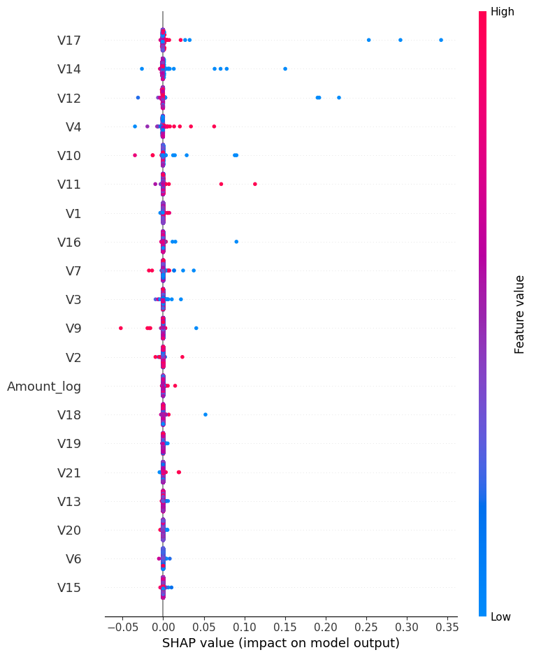
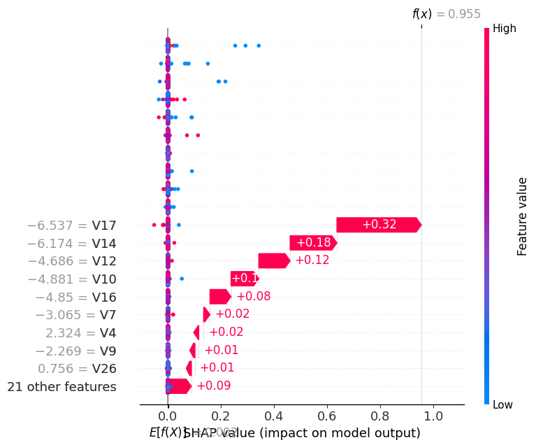
Knowing which features matter on average isn't enough to justify flagging one specific transaction. SHAP attributes each prediction to the individual contribution of every feature, for that exact case.
Five anonymized features — V17, V14, V12, V10, and V16 — consistently dominate the model's fraud predictions, both globally and in individual case breakdowns. For one transaction flagged at 95.5% fraud probability, these five features alone accounted for the large majority of the shift away from the dataset's baseline fraud rate, with the remaining 25 features contributing comparatively little.