The problem
RAVDESS provides 1,440 speech recordings from 24 actors, each portraying one of 8 emotions in a neutral North American accent. The same Mel-spectrogram + ResNet18 recipe that worked well for satellite imagery was applied here — but speech emotion turned out to be a much harder domain shift from natural photographs, and getting a trustworthy result required fixing two real problems along the way, not just tuning hyperparameters.
Key results
From underfitting to overfitting to a workable middle ground
A frozen ResNet18 backbone with only a new linear layer trained (4,104 parameters) underfit the problem — 42.2% train accuracy, actually lower than its 47.6% test accuracy, meaning the model wasn't finding much signal in ImageNet-derived features at all. Unfreezing the last residual block (layer4) with a differential learning rate fixed that, but swung hard the other way: 99.9% train accuracy against just 53.5% test accuracy, memorizing training clips instead of generalizing. SpecAugment — randomly masking frequency and time bands on the training spectrograms only — brought the gap back under control without giving up the accuracy gain.
| Configuration | Train acc | Test acc | Gap |
|---|---|---|---|
| Frozen backbone (linear probe) | 42.2% | 47.6% | underfitting |
| Unfrozen layer4, no augmentation | 99.9% | 53.5% | ~46 pts |
| Unfrozen layer4 + SpecAugment | 80.8% | 64.6% | ~16 pts |
A reproducibility bug, caught before it mattered
While extending training to more epochs, a Colab runtime restart forced the dataset-building step to re-run — and test accuracy unexpectedly jumped, on what looked like a like-for-like re-run. Checking the classification report's per-class support counts revealed the cause: the file-parsing loop listed each actor's audio files without sorting them, so the sample order — and therefore which files landed in train vs. test under a fixed random seed — wasn't guaranteed to stay the same across runs. A one-line fix (sorting the file list) made the split deterministic, and every result reported here was re-verified on that fixed split.
Not the confusion that was expected
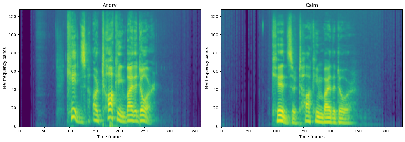
Across every configuration tested, the dominant confusion was sad ↔ calm — not calm ↔ neutral, the pairing initially expected to be hardest to separate. Both sad and calm are low-arousal emotions with flat prosody, and the pattern held even as overall accuracy improved and the underlying test set changed before and after the reproducibility fix — evidence this is a genuine acoustic limit of the pipeline, not noise from one particular split. High-arousal emotions (angry, disgust, surprised) were consistently the easiest to classify, both reaching 75-79% recall in the final model.